Bank & Treasury Management - BSF222Agustin Mackinlay
a.mackinlay@euruni.edu
Session 7 - March 13, 2012
_______________________
. Investment banking: Global Fixed Income League Tables (Bloomberg);
. VIDEO. Tim Bennett on the 5 key activities of investment banks;
. VIDEO: Pictet Private Bank, Geneva, with € 280 billion under management.
Tuesday, March 13, 2012

Tuesday, March 6, 2012
Bank & Treasury Management - BSF222Agustin Mackinlay
a.mackinlay@euruni.edu
Session 6 - March 6, 2012
_______________________
. Banks and the Yield Curve****
[1] DEFINITION
. Frank J. Fabozzi. Fixed Income Mathematics. Anlytical & Statistical Techniques. Chicago: Probus, 1993, chapter 13.
The graphical depiction of the relationship between the yield on securities of the same credit risk and different maturity is called the yield curve. The yield curve is constructed with the maturity and observed yield of Treasury securities because Treasuries reflect the pure effect of maturity alone on yield, given that market participants do not perceive government securities to have any credit risk. When market participants refer to the “yield curve”, they usually mean the Treasury yield curve. This is also true in the bond markets of other countries (P. 218).
Exhibit 13-1 show four yield curves that have been observed in the US Treasury market (and occur in other major government bond markets). In the yield curve in panel a, the yield increases with maturity. This shape is commonly referred to as an upward sloping or normal yield curve. The yield curve on panel b is downward sloping or an inverted yield curve. In a humped yield curve, depicted in panel c of the exhibit, the yield curve initially is upward sloping, but after a certain maturity it becomes downward sloping. Finally, a flat yield curve is one where the yield is the same regardless of the maturity. A flat yield curve is shown in panel d. [COPY OF EXHIBIT 13-1 PROVIDED IN CLASS]

_______________
[2] SOURCES OF INFORMATION
. US Department of the Treasury: Daily Treasury Yield Curve Rates.
. Bloomberg Yield Curves
QUESTIONS : (1) HOW WOULD YOU DEFINE THE SHAPE OF THE YIELD CURVE ON MARCH 12 2004, JANUARY 14 2006, FEBRUARY 27 2007, NOVEMBER 5 2008 AND MARCH 2012?; (2) HOW WOULD YOU CHARACTERIZE THE DIFFERENCE BETWEEN MAY 2004 AND MARCH 2012?]
[3] THE YIELD CURVE AND BANK EARNINGS
[3.1] Definition of Net Interest Margin (*)
Banks have a number of measures, different from those used to analyze industrial companies, that investors can use to evaluate performance. One of the most basic of these is the net interest margin. The net interest margin, also sometimes referred to as the net yield on interest-earning assets, is usually defined as net interest income, divided by average interest-earning assets. The margin is calculated for a period of time, a quarter or a year, and is expressed as a percentage.
NIM = NET INTEREST INCOME / INTEREST-EARNING ASSETS
Net interest income, the numerator of the equation, is the total interest income earned on a bank’s loans, investment securities, and short-term investments (like on interest-bearing deposits with other banks) during a period of time, minus the cost of (interest expense related to) the funds used to make loans and investments. The usual sources of interest-bearing funds include deposits and short- and long-term borrowings.
Average interest-earning assets, the denominator of the ratio, consists of an average of all of a bank’s assets that generate interest income during a specific time period. This excludes certain assets, like property and cash on deposit with the Federal Reserve Bank to meet reserve and clearing requirements, that don’t earn interest income.
Bank balance sheets are often described in terms of their relative responsiveness to changes in short-term interest rates. Banks whose interest-earning assets (loans and investments) tend to reprice more quickly when short-term interest rates change than their interest-bearing deposits and borrowed funds are said to be asset sensitive. They tend to do well when interest rates rise, but their margins are squeezed when short-term interest rates decline. Banks whose liabilities reprice more quickly than their assets are liability sensitive. They probably would have benefited from the decline in short-term interest rates over the 2008 to 2009 period.
(*) From Theresa Brophy: “The Net Interest Margin: What is it? What does it say?”, Value Line, August 2010.
[3.2] Federal Reserve Monetary Policy in the 2000s
. Three-month LIBOR rates: see. [QUESTION: WHAT IS GOING ON? IS THE FEDERAL RESERVE BUYING OR SELLING BONDS TO BANKS? WHY?]
. Raghuram J. Rajan. Fault Lines: How Hidden Fractures Still Threaten the World Economy (Princeton University Press, 2010) [web page] [Introduction] [video]
[3.3] The impact of changes in the yield curve on bank earnings
. FDIC: What the Yield Curve Does (and Doesn’t) Tell Us
Historically, the yield curve spread, or the difference between short-term and long-term interest rates, has had some predictive power for the performance of the U.S. economy and banking industry. In the past, a narrowing, or flattening, of the spread has tended to foretell both slower economic growth and increased pressure on bank earnings. Furthermore, the yield curve generally has inverted—a condition where short-term rates exceed long-term rates—up to two years ahead of a recession. Based on this historical context, the flattening in the yield curve since mid-2004 has been on the minds of many economists and banking analysts.
The Yield Curve and Banks
Just as the yield curve is not a perfect indicator of future economic growth, it also does not provide perfect foresight as to how bank net interest margins (NIMs) and earnings will fluctuate. The traditional view of the banking business holds that banks pay interest on their deposits based upon shorter-term interest rates while making loans tied to longer-term interest rates. Thus, the difference between interest paid and received—the margin—should be influenced by the slope of the yield curve. There is some empirical support for this view.
Large banks tend to have higher concentrations of commercial and industrial (C&I) loans and credit card receivables. The C&I lending environment, especially for large loans exceeding $1 million, has been very competitive in recent years [LOTS OF COMPETITION = ASSETS YIELD LESS]. Not only do banks compete against other banks, but they also compete against capital markets, which have become a popular source of funding for corporations [CORPORATIONS CAN ISSUE BONDS DIRECTLY TO THE MARKET = LESS DEMAND FOR BANK LOANS]. In addition, many corporations have experienced increases in their cash balances in recent years, creating less incentive to reach out to banks for financing [CASH-RICH COMPANIES = LESS DEMAND FOR BANK LOANS]. This strong corporate cash position has weighed on C&I loan growth.
Since early 2004, funding costs at large banks have risen much faster relative to small banks. Large banks have a greater reliance on overnight and wholesale funding than smaller banks. These funds tend to reprice faster than longer-term deposits, such as certificates of deposit and money market accounts, when short-term interest rates rise. This situation has resulted in a classic margin squeeze for the largest banks as the yield curve has flattened.
[3.4] Exercise: The impact of changes in short-term interest rates on Net Interest Margin (NIM)
. LIBOR is at 0.75% at the starting point, at 1.75% in Scenario 1, at 3.75% in Scenario 2;
. Interest paid on Savings accounts does not change (0.5%);
. Interest paid on time deposits is repriced every three-months; assumption: the bank pays 50% of the increase in LIBOR;
. Interest paid on overnight loans from other banks is repriced daily; assumption: the bank pays 100% of the increase in LIBOR;
. Bank A’s Assets. Credit card loans $100 million @ fixed 12%; Adjustable Mortgages (ARMs) $100 million @ LIBOR + 300bps; Fixed-rate mortgages $100 million @ fixed 7%; Floating-rate Bonds $100 million @ LIBOR + 50 bps; Bonds with fixed coupon $100 million @ 4.5%.
. Bank B at starting point; LIBOR = 0.75%.
. Rolfe Winkler: “Yield curve can’t drive profits if banks won’t lend”, Reuters, January 11, 2010. [NICE CHART: NET INTEREST MARGIN AND THE SHAPE OF THE YIELD CURVE]
a.mackinlay@euruni.edu
Session 6 - March 6, 2012
_______________________
. Banks and the Yield Curve****
[1] DEFINITION
. Frank J. Fabozzi. Fixed Income Mathematics. Anlytical & Statistical Techniques. Chicago: Probus, 1993, chapter 13.
The graphical depiction of the relationship between the yield on securities of the same credit risk and different maturity is called the yield curve. The yield curve is constructed with the maturity and observed yield of Treasury securities because Treasuries reflect the pure effect of maturity alone on yield, given that market participants do not perceive government securities to have any credit risk. When market participants refer to the “yield curve”, they usually mean the Treasury yield curve. This is also true in the bond markets of other countries (P. 218).
Exhibit 13-1 show four yield curves that have been observed in the US Treasury market (and occur in other major government bond markets). In the yield curve in panel a, the yield increases with maturity. This shape is commonly referred to as an upward sloping or normal yield curve. The yield curve on panel b is downward sloping or an inverted yield curve. In a humped yield curve, depicted in panel c of the exhibit, the yield curve initially is upward sloping, but after a certain maturity it becomes downward sloping. Finally, a flat yield curve is one where the yield is the same regardless of the maturity. A flat yield curve is shown in panel d. [COPY OF EXHIBIT 13-1 PROVIDED IN CLASS]

_______________
[2] SOURCES OF INFORMATION
. US Department of the Treasury: Daily Treasury Yield Curve Rates.
. Bloomberg Yield Curves
QUESTIONS : (1) HOW WOULD YOU DEFINE THE SHAPE OF THE YIELD CURVE ON MARCH 12 2004, JANUARY 14 2006, FEBRUARY 27 2007, NOVEMBER 5 2008 AND MARCH 2012?; (2) HOW WOULD YOU CHARACTERIZE THE DIFFERENCE BETWEEN MAY 2004 AND MARCH 2012?]
[3] THE YIELD CURVE AND BANK EARNINGS
[3.1] Definition of Net Interest Margin (*)
Banks have a number of measures, different from those used to analyze industrial companies, that investors can use to evaluate performance. One of the most basic of these is the net interest margin. The net interest margin, also sometimes referred to as the net yield on interest-earning assets, is usually defined as net interest income, divided by average interest-earning assets. The margin is calculated for a period of time, a quarter or a year, and is expressed as a percentage.
NIM = NET INTEREST INCOME / INTEREST-EARNING ASSETS
Net interest income, the numerator of the equation, is the total interest income earned on a bank’s loans, investment securities, and short-term investments (like on interest-bearing deposits with other banks) during a period of time, minus the cost of (interest expense related to) the funds used to make loans and investments. The usual sources of interest-bearing funds include deposits and short- and long-term borrowings.
Average interest-earning assets, the denominator of the ratio, consists of an average of all of a bank’s assets that generate interest income during a specific time period. This excludes certain assets, like property and cash on deposit with the Federal Reserve Bank to meet reserve and clearing requirements, that don’t earn interest income.
Bank balance sheets are often described in terms of their relative responsiveness to changes in short-term interest rates. Banks whose interest-earning assets (loans and investments) tend to reprice more quickly when short-term interest rates change than their interest-bearing deposits and borrowed funds are said to be asset sensitive. They tend to do well when interest rates rise, but their margins are squeezed when short-term interest rates decline. Banks whose liabilities reprice more quickly than their assets are liability sensitive. They probably would have benefited from the decline in short-term interest rates over the 2008 to 2009 period.
(*) From Theresa Brophy: “The Net Interest Margin: What is it? What does it say?”, Value Line, August 2010.
[3.2] Federal Reserve Monetary Policy in the 2000s
. Three-month LIBOR rates: see. [QUESTION: WHAT IS GOING ON? IS THE FEDERAL RESERVE BUYING OR SELLING BONDS TO BANKS? WHY?]
. Raghuram J. Rajan. Fault Lines: How Hidden Fractures Still Threaten the World Economy (Princeton University Press, 2010) [web page] [Introduction] [video]
[3.3] The impact of changes in the yield curve on bank earnings
. FDIC: What the Yield Curve Does (and Doesn’t) Tell Us
Historically, the yield curve spread, or the difference between short-term and long-term interest rates, has had some predictive power for the performance of the U.S. economy and banking industry. In the past, a narrowing, or flattening, of the spread has tended to foretell both slower economic growth and increased pressure on bank earnings. Furthermore, the yield curve generally has inverted—a condition where short-term rates exceed long-term rates—up to two years ahead of a recession. Based on this historical context, the flattening in the yield curve since mid-2004 has been on the minds of many economists and banking analysts.
The Yield Curve and Banks
Just as the yield curve is not a perfect indicator of future economic growth, it also does not provide perfect foresight as to how bank net interest margins (NIMs) and earnings will fluctuate. The traditional view of the banking business holds that banks pay interest on their deposits based upon shorter-term interest rates while making loans tied to longer-term interest rates. Thus, the difference between interest paid and received—the margin—should be influenced by the slope of the yield curve. There is some empirical support for this view.
Large banks tend to have higher concentrations of commercial and industrial (C&I) loans and credit card receivables. The C&I lending environment, especially for large loans exceeding $1 million, has been very competitive in recent years [LOTS OF COMPETITION = ASSETS YIELD LESS]. Not only do banks compete against other banks, but they also compete against capital markets, which have become a popular source of funding for corporations [CORPORATIONS CAN ISSUE BONDS DIRECTLY TO THE MARKET = LESS DEMAND FOR BANK LOANS]. In addition, many corporations have experienced increases in their cash balances in recent years, creating less incentive to reach out to banks for financing [CASH-RICH COMPANIES = LESS DEMAND FOR BANK LOANS]. This strong corporate cash position has weighed on C&I loan growth.
Since early 2004, funding costs at large banks have risen much faster relative to small banks. Large banks have a greater reliance on overnight and wholesale funding than smaller banks. These funds tend to reprice faster than longer-term deposits, such as certificates of deposit and money market accounts, when short-term interest rates rise. This situation has resulted in a classic margin squeeze for the largest banks as the yield curve has flattened.
[3.4] Exercise: The impact of changes in short-term interest rates on Net Interest Margin (NIM)
. LIBOR is at 0.75% at the starting point, at 1.75% in Scenario 1, at 3.75% in Scenario 2;
. Interest paid on Savings accounts does not change (0.5%);
. Interest paid on time deposits is repriced every three-months; assumption: the bank pays 50% of the increase in LIBOR;
. Interest paid on overnight loans from other banks is repriced daily; assumption: the bank pays 100% of the increase in LIBOR;
BANK A AND BANK B: BALANCE SHEETS
. Bank A’s Liabilities. Demand deposits $100 million @ zero interest; Savings accounts $100 million @ 0.50%; Time Deposits $100 million @ 2%; Bonds issued by the bank with fixed coupon $100 million @ 4%.
. Bank B’s Assets. Credit card loans $100 million @ fixed 12%; Adjustable Mortgages (ARMs) $100 million @ LIBOR + 300bps; Fixed-rate mortgages $600 million @ fixed 7%; Bonds with fixed coupon $300 million @ 4.5%.
. Bank B’s Liabilities. Demand deposits $100 million @ zero interest; Savings accounts $100 million @ 0.50%; Time Deposits $300 million @ 2%; Floating rate bonds issued by the bank $200 million @ LIBOR + 200 bps; Overnight loans from other banks $300 million @ LIBOR.
QUESTIONS. CALCULATE NET INTEREST MARGIN FOR BANK A AND BANK B AT STARTING POINT AND IN SCENARIOS 1 AND 2].
. Bank A at starting point; LIBOR = 0.75%.
Interest Income = 12.0 +3.75 + 7.00 + 1.25 + 4.5 = 28.5;
Cost of funding = 0.0 + 0.5 + 2.0 + 4.0 = 6.5;
Net Interest Income = 28.5 – 6.5 = 22
NIM = (28.5 – 6.5) / 500 = 4.4%
. Bank A in Scenario 1; LIBOR = 1.75%.
Interest Income = 12.0 + 4.75 + 7 + 2.25 + 4.5 = 30.5;
Cost of funding = 0.0 + 0.5 + 2.5 + 4 = 7.0;
Net Interest Income = 30.5 – 7.0 = 23.5
NIM = (30.5 – 7.0) / 500 = 4.7%
[Note: Time Deposits @ 2% + half the increase in LIBOR = 2% + 0.5% = 2.5%]
. Bank A in Scenario 2; LIBOR = 3.75%.
Interest Income = 12.0 + 6.75 + 7 + 4.25 + 4.5) = 34.5;
Cost of funding = 0.0 + 0.5 + 3.5 + 4.0 = 8.0;
Net Interest Income = 34.5 – 8.0 = 26.5
NIM = (34.5 – 8.0) / 500 = 5.3%
[Note: Time Deposits @ 2% + half the increase in LIBOR = 2% + 1.5% = 3.5%]
Interest Income = 12.0 + 3.75 + 42.00 + 13.5 = 71.25;
Cost of funding = 0.0 + 0.5 + 6.0 + 5.5 + 2.25 = 14.25;
Net Interest Income = 71.25 – 14.25 = 57.0
NIM = (71.25 – 14.25) / 1100 = 5.2%
. Bank B in Scenario 1; LIBOR = 1.75%.
Interest Income = 12.0 + 4.75 + 42 + 13.5 = 72.25;
Cost of funding = 0.0 + 0.5 + 7.5 + 7.5 + 5.25 = 20.75;
Net Interest Income = 72.25 – 20.75 = 51.50
NIM = (72.25 – 20.75) / 1100 = 4.7%
[Note: Time Deposits @ 2% + half the increase in LIBOR = 2% + 0.5% = 2.5%]
. Bank B in Scenario 2; LIBOR = 3.75%.
Interest Income = 12.0 + 6.75 + 42 + 13.5 = 74.25;
Cost of funding = 0.0 + 0.5 + 10.5 + 11.5 + 11.25 = 33.75;
Net Interest Income = 74.25 – 33.75 = 40.5
NIM = (74.25 – 33.75) / 500 = 3.7%
[Note: Time Deposits @ 2% + half the increase in LIBOR = 2% + 1.5% = 3.5%]
QUESTIONS & DEBATE
Identify fixed rate assets and liabilitiesIdentify floating rate assets and liabilities
Which bank is more affected by an interest rate increase?
Which bank is ‘asset sensitive’, which bank is ‘liability sensitive’?
Could we expect that the larger the interest rate increase, the larger the impact on NIM in Bank B?
What strategy can Bank B implement to diminish interest rate sensitiveness? From the FDIC article: “On top of an increased reliance on fee and other non-interest income, banks have additional means to reduce the impact of yield curve changes on profits. For example, many banks, especially the large ones, have been able to hedge their interest rate exposure by using derivatives.”
What would happen to NIM in Bank A and Bank B in case of an interest rate decline?
What is the purpose of Banco Santander’s campaign offering LED TV 26 inches for customers that bring their payroll to the bank?
Why would certain central banks (Bank of Canada and Sweden’s Riksbank) always endeavor to avoid drastic changes in the shape of the yield curve? Can they accomplish that a goal? How?
The FDIC paper: “Large banks have a greater reliance on overnight and wholesale funding than smaller banks. These funds tend to reprice faster than longer-term deposits, such as certificates of deposit and money market accounts, when short-term interest rates rise”. Does this apply to Bank A or Bank B?
Apply the NIM framework to the 2007-2008 financial crisis, where banks and investment banks financed massive long-term mortgage assets of questionable quality with mostly overnight loans.
A comment by Larry Fink: “European banks have preferred to borrow only short-term money because the interest rates tended to be cheaper. But that has exposed them to the risk that when they try to roll over their debts, the markets may balk” (Financial Times, November 26, 2010). What do you think?
UBS E-News for Banks, January 2012. Executive Summary. The performance of the global banking sector was one of the poorest in recorded history. In 2011, global banks’ performance was down 21.0% in absolute terms and 14.6% lower on a relative basis. Only in 2008, at the height of the global financial crisis, did the sector perform more poorly (see Chart 1). In our opinion, the poor performance – both absolute and relative – can be attributed to a combination of rising macroeconomic uncertainties, spill-over risks and contagion fears arising out of the European sovereign crisis, and persistent regulatory risks, notably at the national level. Increased risk aversion, arising from market concerns over the global economic outlook and notably Europe’s sovereign crisis has also undermined client activity levels and trading volumes, and, together with prevailing low interest rates and flattish yield curves, has weighed on revenues and earnings. [QUESTION: PLEASE EXPLAIN THIS LAST POINT]
[4] REVIEWING THE EVIDENCE
. Federal Reserve Bank of New York: The Yield Curve as a Leading Indicator. [The New York Fed estimates the probability of a US recession according to the shape of the yield curve. How would you rate that probability, given the shape of the yield curve?]
. Rolfe Winkler: “Yield curve can’t drive profits if banks won’t lend”, Reuters, January 11, 2010. [NICE CHART: NET INTEREST MARGIN AND THE SHAPE OF THE YIELD CURVE]
. US Banks: Nonperforming Total Loans;
. US Banks: Net Interest Margin for all U.S. Banks (USNIM)
_______________
Monday, February 27, 2012

Agustin Mackinlay
a.mackinlay@euruni.edu
Session 5 - February 28, 2012
_______________________
· A word on the TED spread**
· Credit markets***, Flight-to-quality****, Funding***, Central bank liquidity operations***, Eurodollar futures***: a review
A word on the TED spread**
. Mark Gonglof: “TED Spread Hits Highest Level Since Crisis”, Wall Street JournalThe Ted spread [chart] is a difference between two short-term interest rates. It is watched anxiously (in times of Flight-to-Safety) by bank managers. The TED spread is the difference between the three-month LIBOR rate and the yield of the three-month Treasury bill. It is currently at about 36 basis points:
TEDspread = 0.45% [LIBOR RATE] – 0.09% [TREASURY BILL RATE] = 0.36%
The TED spread is a measure of the overall confidence in the banking system. When confidence is high, the TED spread is low: banks have little or no funding problems, and depositors feel that their more money is safe. During a F-t-Q episode, however, funding problems arise; LIBOR rates go up as depositors demand higher deposit rates and banks do not trust each other in the money market; this pushes LIBOR higher (less supply of credit). At the same time, savers worry about the return of their money, no about the return on their money. The park money in short-term Treasury Bills, widely considered one of the safest and most liquid assets in the world. This pushes T-Bill rates down (more supply of credit).
[QUESTION: HOW WOULD YOU PLAY THE TED SPREAD IN THE FUTURES MARKET, ASSUMING THAT THE T-BILL FUTURES ARE STRUCTURED JUST AS THE EURODOLLAR FUTURES?]
________________
Credit markets***, Flight-to-quality****, Funding***, Central bank liquidity operations***, Eurodollar futures***. A ‘dynamic’ review of the issues
[1] The Role of the Dollar. Understanding the banking crisis: a (brief) look at the US dollar as the key international reserve currency. 1945-1973: Germany & Japan; 1978-2007: China. The stock of productive capital destroyed; authoritarian political culture. The solution: LOW COST OF LABOUR through a fixed (and undervalued) local currency exchange rate against the dollar.
[2] China’s economic development model. In order to avoid an exchange rate adjustment, China recycles its foreign-exchange reserves into the US credit market. [QUESTION: IMPACT ON THE US CREDIT MARKET??][CHART] [Annex to the Federal Reserve’s Weekly Balance Sheet]. Michael P. Dooley, David Folkerts-Landau & Peter Garber: “An Essay on the Revived Bretton Woods System”, NBER Working Paper 9971 (2003).
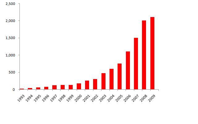
[3] Psychology & Markets: Attitudes toward risk. US credit markets flooded with cash! Jacques Rueff. Le péché monétaire de l’Occident. Paris: Plon, 1971: “The process works this way. When the U.S. has an unfavorable balance with another country (let us take as an example France), it settles up in dollars. The Frenchmen who receive these dollars sell them to the central bank, the Banque de France, taking their own national money, francs, in exchange. The Banque de France, in effect, creates these francs against the dollars. But then it turns around and invests the dollars back into the U.S. Thus the very same dollars expand the credit system of France, while still underpinning the credit system in the U.S. The country with a key currency is thus in the deceptively euphoric position of never having to pay off its international debts. The money it pays to foreign creditors comes right back home, like a boomerang … The functioning of the international monetary system is thus reduced to a childish game in which, after each round, the winners return their marbles to the losers … The discovery of that secret [namely, that no adjustment takes place] has a profound impact on the psychology of nations (la psychologie des peuples) … This is the marvelous secret of the deficit without tears, which somehow gives some people the (false) impression that they can give without taking, lend without borrowing, and purchase without paying. This situation is the result of a collective error of historic proportions”
[4] Psychology & Markets: Attitudes toward risk
F = 2.5 x G !!!
Some references on emotions, the economy, credit markets:
Some references on emotions, the economy, credit markets:
. Akerlof, George A. & Schiller, Robert A. Animal Spirits. How Human Psychology Drives the Economy, and Why it Matters for Global Capitalism (Princeton University Press, 2009) [see]
. Gasparino, Charles. The Sellout. How Three Decades of Wall Street Greed and Government Mismanagement Destroyed the Global Financial System (New York: HarperBusiness, 2009) [see]. From a Financial Times review: “Gasparino narrates convincingly how banks such as Bear [Stearns] slipped into risking ever more capital, often without the full understanding of their leaders, who were engaged in a contest to see who could catch up with Goldman Sachs”. The same, by the way, could be said about Swiss bank UBS.
. Tett, Gillian: “The emotional markets hypothesis and Greek bonds”, Financial Times, April 10/11 2010.
. Turner Review. A regulatory response to the global banking crisis (London: Financial Services Authority, 2009). See p. 41: “Individual behaviour is not entirely rational. There are moreover insights from behavioural economics, cognitive psychology and neuroscience, which reveal that people often do not make decisions in the rational front of brain way assumed in neoclassical economics, but make decisions which are rooted in the instinctive part of the brain, and which at the collective level are bound to produce herd effects and thus irrational momentum swings”.
. J. M. Coates & J. Herbert: “Endogenous steroids and financial risk taking on a London trading floor”, Proceedings of the National Academy of Sciences, April 2008 [Judge Business School, University of Cambridge, Cambridge CB2 1AG, United Kingdom ; Cambridge Center for Brain Repair, University of Cambridge, Cambridge CB2 0PY, United Kingdom]. Edited by Bruce S. McEwen, The Rockefeller University, New York, NY, and approved November 6, 2007 (received for review May 1, 2007)
Abstract
Little is known about the role of the endocrine system in financial risk taking. Here, we report the findings of a study in which we sampled, under real working conditions, endogenous steroids from a group of male traders in the City of London. We found that a trader's morning testosterone level predicts his day's profitability. We also found that a trader's cortisol rises with both the variance of his trading results and the volatility of the market. Our results suggest that higher testosterone may contribute to economic return, whereas cortisol is increased by risk. Our results point to a further possibility: testosterone and cortisol are known to have cognitive and behavioral effects, so if the acutely elevated steroids we observed were to persist or increase as volatility rises, they may shift risk preferences and even affect a trader's ability to engage in rational choice.
. Roger Boyes: "Age of Testosterone comes to end in Iceland", TimesOnline (February 7, 2009). Iceland, ravaged throughout history by volcanic eruptions and natural catastrophes, is struggling with a man-made disaster so overwhelming that the women are taking over. It is, they say here, the end of the Age of Testosterone. Next week a newly minted left-leaning Government led by Johanna Sigurdardottir will start to tackle the tough agenda of cleaning out the old-school-chum networks that have led Iceland to the verge of bankruptcy. Half of her Cabinet will be women; female advisers carrying briefcases move in and out of the Prime Minister's whitewashed office, a former jailhouse in the middle of Reykjavik. Two women, Birna Einarsdottir and Elin Sigfusdottir, now run the struggling and disgraced New Landsbanki and New Glitnir banks. We have to create a new sense of solidarity,” says the Social Democrat Prime Minister. The departing Government — retreating would be more precise — put business first, people second, say the premier's counsellors. Now is the time for a shift in values. Listening to Ms Sigurdardottir talk in her dry, schoolmistress manner, it becomes clear that the fall of the Icelandic Government was not just the first political casualty of the global downturn, but also a signal that men in suits have led the world astray. “We are going to base our economic policies on prudence and responsibility, but we also stress social values, women's rights, equality and justice,” she says. “You can see what is happening,” says Katrin Olafsdottir, Associate Professor of Economics and a member of the board of New Glitnir, which is trying to devise a new mission for the crippled bank. “The men went out there and took these incredibly irrational risks — and getting loads of money for doing it, feeling really good about it - and then the women have to come in to clean it up.”
. Gasparino, Charles. The Sellout. How Three Decades of Wall Street Greed and Government Mismanagement Destroyed the Global Financial System (New York: HarperBusiness, 2009) [see]. From a Financial Times review: “Gasparino narrates convincingly how banks such as Bear [Stearns] slipped into risking ever more capital, often without the full understanding of their leaders, who were engaged in a contest to see who could catch up with Goldman Sachs”. The same, by the way, could be said about Swiss bank UBS.
. Tett, Gillian: “The emotional markets hypothesis and Greek bonds”, Financial Times, April 10/11 2010.
. Turner Review. A regulatory response to the global banking crisis (London: Financial Services Authority, 2009). See p. 41: “Individual behaviour is not entirely rational. There are moreover insights from behavioural economics, cognitive psychology and neuroscience, which reveal that people often do not make decisions in the rational front of brain way assumed in neoclassical economics, but make decisions which are rooted in the instinctive part of the brain, and which at the collective level are bound to produce herd effects and thus irrational momentum swings”.
. J. M. Coates & J. Herbert: “Endogenous steroids and financial risk taking on a London trading floor”, Proceedings of the National Academy of Sciences, April 2008 [Judge Business School, University of Cambridge, Cambridge CB2 1AG, United Kingdom ; Cambridge Center for Brain Repair, University of Cambridge, Cambridge CB2 0PY, United Kingdom]. Edited by Bruce S. McEwen, The Rockefeller University, New York, NY, and approved November 6, 2007 (received for review May 1, 2007)
Abstract
Little is known about the role of the endocrine system in financial risk taking. Here, we report the findings of a study in which we sampled, under real working conditions, endogenous steroids from a group of male traders in the City of London. We found that a trader's morning testosterone level predicts his day's profitability. We also found that a trader's cortisol rises with both the variance of his trading results and the volatility of the market. Our results suggest that higher testosterone may contribute to economic return, whereas cortisol is increased by risk. Our results point to a further possibility: testosterone and cortisol are known to have cognitive and behavioral effects, so if the acutely elevated steroids we observed were to persist or increase as volatility rises, they may shift risk preferences and even affect a trader's ability to engage in rational choice.
. Roger Boyes: "Age of Testosterone comes to end in Iceland", TimesOnline (February 7, 2009). Iceland, ravaged throughout history by volcanic eruptions and natural catastrophes, is struggling with a man-made disaster so overwhelming that the women are taking over. It is, they say here, the end of the Age of Testosterone. Next week a newly minted left-leaning Government led by Johanna Sigurdardottir will start to tackle the tough agenda of cleaning out the old-school-chum networks that have led Iceland to the verge of bankruptcy. Half of her Cabinet will be women; female advisers carrying briefcases move in and out of the Prime Minister's whitewashed office, a former jailhouse in the middle of Reykjavik. Two women, Birna Einarsdottir and Elin Sigfusdottir, now run the struggling and disgraced New Landsbanki and New Glitnir banks. We have to create a new sense of solidarity,” says the Social Democrat Prime Minister. The departing Government — retreating would be more precise — put business first, people second, say the premier's counsellors. Now is the time for a shift in values. Listening to Ms Sigurdardottir talk in her dry, schoolmistress manner, it becomes clear that the fall of the Icelandic Government was not just the first political casualty of the global downturn, but also a signal that men in suits have led the world astray. “We are going to base our economic policies on prudence and responsibility, but we also stress social values, women's rights, equality and justice,” she says. “You can see what is happening,” says Katrin Olafsdottir, Associate Professor of Economics and a member of the board of New Glitnir, which is trying to devise a new mission for the crippled bank. “The men went out there and took these incredibly irrational risks — and getting loads of money for doing it, feeling really good about it - and then the women have to come in to clean it up.”
[5] Vulnerabilities, 2007-2008
. Tim Geithner: “A Disaster Far Beyond Lehman Brothers Collapse”, Banking & Finance News, 20 April 2010.
. Raghuram J. Rajan. Fault Lines: How Hidden Fractures Still Threaten the World Economy (Princeton University Press, 2010) [web page] [Introduction] [video]
. Ann O’Ryna Spehar: “The Great Moderation and the Business Cycle”, MPRA Paper No. 12274, December 2008.
The size of the SHADOW BANKING SYSTEM. By 2007, the US banking system had seen enormous change. Instead of focusing on old-fashioned banking and holding mortgage loans on their books, many banks became like sausage factories: originate mortgages, then sell them to investors and to … their own off-balance investment vehicles. US Treasury Secretary Tim Geithner: “In the run-up to the recent crisis, we witnessed a period of explosive growth in leverage and maturity transformation outside the perimeter of prudential banking regulation. This parallel, lightly regulated system has come to be known as the “shadow banking system.” Large dealer firms like Lehman were a key part of this system–but they were just one part. At its peak, the shadow banking system financed about $8 trillion in assets with short-term obligations, making it almost as large as the real banking system”.The rate of home ownership almost reaches 70% in 2006.
Why and how? WHY? (1) to achieve hedge fund link returns through leverage; (2) to get big bonuses!; (3) to achieve too-big-to-fail status.
The Asset / Liability Mismatch problem. While it is a natural occurrence in banking, it took unusual proportion during the 2002-2007 years. Largely driven by THE BELIEF THAT INTEREST RATES WERE STAYING LOW FOREVER, Special Investment Vehicles belonging to banks bought long-term, high-yielding subprime mortgage-backed securities with short-term debt instruments from money market funds. Some banks achieved 30-1 leverage ratios! It proved very profitable between 2003 and 2006.
. Sources of risk. We can see 2 sources of risk: (a) a fall in the value of the assets (mortgage-backed securities); (b) a rise in the cost of short-term credit. By 2007, banks were financing mortgage-backed securities with very short-term debt – based on the belief that interest rates would stay low.
. Fed raises short-term interest rates. Starting in mid-2004, the Federal Reserve raises its target rate for the interest rate at which banks lend to each other, from 1% (following the terrorist attacks of 2001) to 5.25%, because of fears of rising inflation expectations.[CHART]
. Disaster strikes in early and mid-2007. DEFAULT RATES GO UP in the subprime mortgage loan market! They reach 20%, as the job market deteriorates. The news sends the market in turmoil. WHAT ARE THE ALTERNATIVES AT THAT STAGE? [Simulation: sell assets / raise capital / take losses and close down operations / take SIVs back into the balance sheet of the bank].
Assets CITIGROUP : SIVs & CONDUITS Liabilities & Capital
. Mortgage-backed securities: $ 156 billion ( high interest rate: 12%, but very long-term) | |
. Short-term credit: $ 144 billion ( low interest rate: 3%, but very short-term) | |
. Capital: $ 12 billion |
Assets CITIGROUP : SIVs & CONDUITS Liabilities
THE VALUE OF THE ASSETS (SUBPRIME MORTGAGE-BACKED SECURITIES) IS …. COLLAPSING! (1) | THE COST OF FINANCING THE ASSETS (SUBPRIME MORTGAGE-BACKED SECURITIES) IS …. SOARING! (2) |
(1) Because rising unemployment has suddenly created a wave of defaults amid subprime mortgage borrowers!
(2) Because the Federal Reserve –fearing the prospect of higher inflation rates– has been increasing the target rate for the rate at which banks lend to each other.
[6] The Lehman Brothers collapse, September 15 2008
Lehman Brothers, one of the oldest Wall Street investment banks, was holding as much as $327 billion in assets (including subprime mortgage-backed securities), of which at least $50 billion in subprime mortgage-backed securities had been hidden from view. By September 2008, its losses were of such magnitude that it had not enough capital to cover them. The day it is finally declared bankrupt (September 15), it was owing $613 billion in debt. Panic in money markets!
Panic in interbank lending markets!
[7] FLIGHT-TO-QUALITY!****
See blog post for Session 2:
[8] TED spread soars!***
Banks in the US and Europe are having serious funding problems. Witness: the TED spread.
[9] Central banks ease monetary policy
. Federal Reserve: Credit and Liquidity Programs and the Balance Sheet
As demand for credit declines, the rate at which banks lend to each other starts to decrease. Central banks have two possibilities. Either they announce a new (LOWER) target rate, or the sell bonds to commercial banks in order to drain liquidity [CHART] [ECB target rates].

See Session 3.
Nicolas Sarkozy and the ECB.
[10] First round of Central banks liquidity swaps***
. Federal Reserve: Central Bank Liquidity Swaps
To prevent the flight-to-quality to spread further, central banks launch the first series of highly successful CENTRAL BANK LIQUIDITY SWAPS.
See session 4.
No central bank liquidity swaps for Ms. Tymoshenko’s Ukraine!
[11] The Federal Reserve implements Quantitative Easing (QE)
. Federal Reserve: Central Bank Liquidity Swaps
The target rate for overnight loans between banks is lowered to … zero. Reserves of commercial banks at the Federal Reserve reach US$1 trillion. [CHART].
[DIAGRAM]
[12] Greece cooks the books: a new round of Flight-to-Quality. Assets & Liabilities at European banks***
As the Greek government informs that it had ‘cooked the books’, a new round of F-t-Q begins. This time, the epicenter is … Europe. The process goes on, with ups and downs, from 2009 to 2011. All indicators of F-t-Q start to flash: credit spreads, banks’ stock prices, the TED spread.
[HOW DOES IT AFFECT EUROPEAN BANKS? THINK IN TERMS OF ASSETS, LIABILITIES ]
See session 4.
[13] November 30, 2011. Second round of Central Bank Liquidity Swaps. European banks need funding in US$ dollars!***
ECB announcement.
See session 4.
[14] December 22, 2011. The European Central Bank announces first tranche of Long-Term Refinancing Operations***
See session 3.
Show me the money! [video].
[15] February 29, 2012. The European Central Bank announces second tranche of Long-Term Refinancing Operations
_____________
.jpg/250px-Chicago_Mercantile_Exchange_(G._Bush).jpg)
Agustin Mackinlay
a.mackinlay@euruni.edu
Session 5 - February 28, 2012
__________________________________
From chapter 6 of John C. Hull. Options, Futures, and Other Derivatives, sixth edition, 2005.
EURODOLLAR FUTURES
The most popular interest rate futures contract in the United States is 3-month Eurodollar futures contract traded on the Chicago Mercantile Exchange (CME). A Eurodollar is a dollar deposited in a US or foreign bank outside the United States. The Eurodollar interest rate is the rate of interest earned on Eurodollars deposited by one bank with another bank. It is essentially the same as the London Interbank Offer Rate (LIBOR).
Three-month Eurodollar futures contracts are futures contracts on the 3-month (90-day) Eurodollar interest rate. They allow an investor to lock in an interest rate on $1 million for a future 3-month period. The 3-month period to which the interest rate applies starts on the third Wednesday of the expiration month. The contracts have expiration months of March, June, September and December for up to ten years into the future. This means that in 2004 an investor can use Eurodollar futures to lock in an interest rate fpr 3-month periods that are as far into the future as 2014.
To understand how Eurodollar futures contracts work, consider the March 2005 contract. This has a settlement price of 97.63. The contract ends on the third Wednesday of the expiration month. The contract is marked to market in the usual way until that date. On March 16, the settlement price is set equal to 100 – I, where i is the actual 3-month Eurodollar interest rate on that day, expressed with quarterly compounding and an actual/360 day count convention. (Thus, if the 3-month Eurodollar interest rate on March 16, 2005, turned out to be 2%, the final settlement price would be 98). There is a final marking to market reflecting the settlement price and all contracts are declared closed.
The contract is designed so that a 1 basis point (=0.01) move in the futures quote corresponds to a gain or loss of $25 per contract. When a Eurodollar futures quote increases by one basis point, a trader who is long one contract gains $25 and a trader who is short one contract loses $25. Similarly, when the quote decreases by one basis point, a trader who is long one contract loses $25 and a trader who is short one contract gains $25. This is consistent with the point made earlier: that the contract locks in an interest rate on $1 million dollars for 3 months. When an interest rate per year changes by one basis point, the interest earned on 1 million dollar for three months changes by
1,000,000 x 0.0001 x 0.25 = 25
or $25. Because the futures quote is 100 minus the futures interest rate, an investor who is long gains when interest rates fall and an investor who is short gains when interest rates rise.
Example
On February 4, 2004, an investor wants to lock in the interest rate that will be earned on $5 million for 3 months starting on March 16, 2005. The investor goes long five March05 Eurodollar futures contracts at 97.63. On March 16, 2005, the 3-mont LIBOR interest rate is 2%, so that the final settlement price proves to be 98.00. The investor gains 5 x 25 x [(98.00 – 97.63) x 100] = $4,625 on the long futures position. The interest earned on the $5 million for three months is
5,000,000 x 0.25 x 0.02 = 25,000
or $25,000. The gain on the futures contract brings this up to $29,625. This is the interest that would have been earned if the interest rate had been 2.37% (5,000,000 x 0.25 x 0.0237 = 29,625). The illustration shows that the futures trade has the effect of locking in an interest rate equal to 2.37%, or (100 – 97.63)%.
The Chicago Mercantile Exchange defines the contract price as
10,000 [100 – 0.25(100 – Q)]
Where Q is the quote. Thus the settlement price of 97.63 for the March 2005 corresponds to a contract price of
10,000 [100 – 0.25(100 – 97.63)] = $994,075
In our example the final price is
10,000 [100 – 0.25(100 – 98.00)] = $995,000
and the difference between the initial and the final contract price is $925, so that an investor with a long position in five contracts gains 5 x 925 dollars, or $4,625 as in the example. This is consistent with the “$25 per 1 basis point move” rule.
_________________
Tuesday, February 21, 2012
Bank & Treasury Management - BSF222
Agustin Mackinlay
a.mackinlay@euruni.edu
Session 4 - February 21, 2012
__________________________________
Central Bank Liquidity Swaps
- A very recent topic. No discussion in textbooks!
- [VIDEO].
- [VIDEO] Ben Bernanke, the Fed chairman, on swaps. Very nervous!
- The latest round of central bank liquidity swaps was announced on November 30, 2011 [see].
- We can check the numbers by looking at the Federal Reserve’s weekly balance sheet.
- October 29, 2008: Fed and central banks of Brazil, Mexico, Singapore and South Korea ($30bn each).
- CHART BRAZIL 5-YEAR CDS
An introduction to Eurodollar futures****
- Chicago Mercantile Exchange: Contract Specifications
- Eurodollar futures are a complete misnomer: they refer to the LIBOR interest rate, not to the €/$ exchange rate between the currencies. The LIBOR rate is the rate at which banks lend to each other; it is heavily influenced by the ‘target’ rate set by the central bank.
- Eurodollar futures are an exchange-traded product, as opposed to an over-the-counter market. The clearing house is the Chicago Mercantile Exchange; see Contract Specifications
- CHART: US monetary base; CHART: US Banks reserves at the Federal Reserve
__________________
Agustin Mackinlay
a.mackinlay@euruni.edu
Session 4 - February 21, 2012
__________________________________
Central Bank Liquidity Swaps
- A very recent topic. No discussion in textbooks!
- [VIDEO].
- [VIDEO] Ben Bernanke, the Fed chairman, on swaps. Very nervous!
- The latest round of central bank liquidity swaps was announced on November 30, 2011 [see].
- We can check the numbers by looking at the Federal Reserve’s weekly balance sheet.
- October 29, 2008: Fed and central banks of Brazil, Mexico, Singapore and South Korea ($30bn each).
- CHART BRAZIL 5-YEAR CDS
An introduction to Eurodollar futures****
- Chicago Mercantile Exchange: Contract Specifications
- Eurodollar futures are a complete misnomer: they refer to the LIBOR interest rate, not to the €/$ exchange rate between the currencies. The LIBOR rate is the rate at which banks lend to each other; it is heavily influenced by the ‘target’ rate set by the central bank.
- Eurodollar futures are an exchange-traded product, as opposed to an over-the-counter market. The clearing house is the Chicago Mercantile Exchange; see Contract Specifications
- CHART: US monetary base; CHART: US Banks reserves at the Federal Reserve
__________________
Subscribe to:
Posts (Atom)